Exhaustive Search

My program for finding 2LBB Busy Beavers can be found on github. This page explains why this search is hard and describes several tricks used by the search program.

Combinatorial explosion

Searching for Busy Beavers is hard because of the combinatorial explosion. There are two problems.

First, the number of possible programs increases exponentially with the size of the grid. For an n×n grid, there are 3^n² possible programs.

Second, the run length also increases. In fact, I expect the maximum run length to increase more than exponentially. Although I have not yet read the proof for the non-computability of Turing-Machine Busy Beavers, I assume the same reasoning can be applied to 2LBB programs as there is no fundamental difference. This would mean that the maximum run length is a non-computable function. At any rate, the time required to evaluate individual programs goes up quickly for increasing grid sizes.

So it is clear that there are limits to the Busy Beavers that can be found. Various optimizations can, however, speed up the search significantly.

Ignore "Don't Care" instructions

Many programs are effectively the same. For a given program the program pointer (PP) only visits a subset of cells on the grid. For the cells it does not visit, it does not matter what instruction they contain. So an important optimization is to not evaluate multiple programs that only differ in these "Don't Care" instructions.

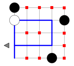
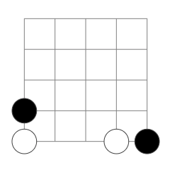
Figure 1 shows these Don't Care instructions for an example program. This program has eleven Don't Care instructions. By ignoring these, for this program alone, the search skips needless evaluation of 3¹¹ - 1 programs.

Ignoring Don't Cares can be done by letting the search lazily instantiate instructions: an instruction is instantiated when it is first encountered during program execution. So program execution and search are combined. As Don't Care cells are not visited, they remain unset. The pseudo-code below illustrates the basic idea. It is optimized for clarity, not performance.

// The recursively growing program
Program program

// Execution state: data, Program Pointer, number of steps
ExecutionState execState

function branch():
  for ins in [NOOP, DATA, TURN]:
    ExecutionState execState0 = execState.copy()
    program[execState.pp] = ins
    run()
    execState = execState0
  program[execState.pp] = UNSET

function run():
  while true:
    ins = program[execState.pp]
    switch ins:
      case UNSET:
        branch()
        return
      case DONE:
        reportDone(program, execState)
        return
      default:
        // Updates PP, Data and numSteps
        execState.execute(ins)

Table 1 gives an indication of the speed up that is achieved. The second column lists the total number of possible programs. The third column gives the total number of distinct programs, after ignoring Don't Care instructions. The actual speed up is obviously less than the ratio of both these numbers as the recursion entails some cost. In particular, an undo history needs to be maintained for all operations that modify state, including changes to the data tape. Nevertheless, these extra costs are clearly outweighed by the huge reduction in the number of programs to evaluate.

**Table 1.** Comparison of the number of programs to evaluate when ignoring Don't Care instructions
Size	#Programs (Total)	#Programs (Ignoring Don't Cares)
3×3	2.0 · 10⁴	59
4×4	4.3 · 10⁷	8.9 · 10²
5×5	8.5 · 10¹¹	6.0 · 10⁴
6×6	1.5 · 10¹⁷	1.9 · 10⁷

**Figure 1.** The instructions at the red cells are Don't Cares

Ignore equivalent DATA permutations

For DATA instructions that are encountered before the first TURN, their exact location does not matter. It only matters how many there are. This follows from the fact that these instructions are only evaluated once, right at the start of the program, and at most once more, just before the program terminates.

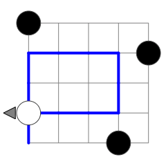
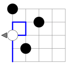
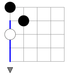
For example, Figure 2 shows a program that is effectively the same as the one in Figure 1. The DATA instruction could be moved to any cell underneath the TURN instruction in the first column without impacting the run length of this program (or any other possible program with the same start). Figure 3 and 4 show the only ways in which instructions that are executed before the first TURN can be executed twice. Whether PP passes through such an early DATA instruction for a second time does not impact execution length.

When the first TURN is the second instruction that is executed, PP traverses the bottom row. Here similarly the location of DATA instructions before the second TURN does not matter, only their number. Figure 5 shows an example. Where the second DATA instruction is placed on the bottom row does not impact execution length of any of the possible programs that may follow the second TURN.

Table 2 shows how ignoring these equivalent DATA permutations further reduces the search space. For the grid sizes shown the reduction in size is approximately a factor two, and will go up for larger grid sizes. Although the speed up is relatively small compared to the previous improvement there is no performance penalty associated with it. It is also straightforward to implement so there is no reason not to also implement this improvement.

**Table 2.** Comparison of the number of programs to evaluate when also ignoring equivalent DATA permutations
Size	#Programs (Only ignoring Don't Cares)	#Programs (Also ignoring Data Permutations)
3×3	59	31
4×4	8.9 · 10²	5.2 · 10²
5×5	6.0 · 10⁴	3.1 · 10⁴
6×6	1.9 · 10⁷	8.0 · 10⁶

**Figure 2.** A program that is run-length equivalent to the program in Figure 1

**Figure 3.** Case 1 where an early DATA instruction is executed twice

**Figure 4.** Case 2 where an early DATA instruction is executed twice

**Figure 5.** Equivalent DATA placement on the bottom row

"On the fly" interpretation

In order to speed up execution and to facilitate hang detection, the generated 2L programs are interpreted on the fly. Instead of moving PP one step at a time, the program is converted into Program Blocks.

A Program Block always contains one or more DATA instructions. It ends at the first TURN that follows a DATA instruction. This implies that when the block contains multiple DATA instructions, they all evaluate to the same operation. A block can contain multiple TURNs. These extra TURN instructions then occur before the first DATA instruction.

The interpreted program for the program in Figure 5 is as follows:

0: INC 3 => -/1
1: SHR 1 => 2/3
2: INC 1 => -/4
3: SHL 1 => EXIT
4: DEC 1 => 5/6
5: SHL 1 => 7/4
6: SHR 1 => 5/6
7: DEC 1 => -/3

Each line is a program block. From left to right it consists of the following:

A unique ID
The operation to carry out
The next program block to execute. When the data value at DP is zero, the first block should be executed, otherwise the second

Also associated with each block, but not shown, is the number of PP execution steps it represents.

Some blocks only have one possible continuation. This is the case when they are entered with a zero value and carry out a INC or DEC operation. In this case the value is always non-zero at the end of the block.

As the program grid is generated on the fly by the search, program blocks can have two states:

Pending: Its operation and continuation program blocks are still unset. This happens when the program block depends on a program cell that is still unset.
Finalized: Its operation and continuation program blocks are set.

A block is finalized as soon as its operation is known. Its continuation program blocks are then also set. These may already exist, but if not, will be created. In both cases, their state can be Pending or Finalized.

Figure 6. The 5×5 Busy Beaver (43 steps)

Hang detection

It is also important to automatically detect hangs. Without doing so the search can only "assume" that a program hangs when its execution exceeded a pre-configured number of steps. Using this cut-off limit is problematic for two reasons. First, it slows down the search. This is especially the case when this limit is high, which it needs to be for bigger grids. Second, it also risks missing the Busy Beaver or a Busy Beaver Champion. This happens when the cut-off limit is lower than the run length of the program.

Detecting all possible hangs is equivalent to solving the Halting Problem, which is known to be impossible. However, as long as a program is "simple enough" it is possible to automatically determine when it hangs.

Static analysis

Many hangs can be detected via static analysis of the interpreted program. This boils down to a single detection algorithm:

No Exit Hang Detection

Dynamic analysis

For hangs that cannot be detected statically, dynamic analysis can be used. Here the behaviour of the program is observed while it is being executed. Dynamic analysis considers has two main inputs:

How data changes over time
How program execution varies over time

Dynamic analysis currently recognizes and detects the following types of hangs:

Phased search

On 7×7 grids and larger the possible execution length of programs goes up rapidly. To account for that a phased search approach is used.

Initially, hang detection is enabled and the search recursively expands the program as it is being evaluated. This is the phase during which the large majority of possible programs is classified. They either terminate relatively quickly or are detected to be hanging.

Hang detection, however, incurs a performance penalty and uses memory to store required run history and data snapshots. At a certain stage this is not effective anymore. Either the program will terminate successfully, in which case hang detection is only slowing down execution, or the program hangs but then it's unlikely that the hang will be automatically detected by the current hang detection logic, given that it has not yet done so. For these reasons hang detection is disabled once the program execution passed a certain configured number of execution steps.

The actual implementation of the search program for rewinding execution state is different than the pseudo-code shown above. It tracks individual data operations and undoes these. This is more efficient early on in the search, when search space branches quickly which involves considerable backtracking. However, it incurs fixed execution overhead per data operation and the required memory grows linearly with the program's execution length. Therefore, at a certain stage this is not effective anymore either and also disabled.

Once backtracing is disabled, that part of the search space cannot be expanded further. Instead, the search switches to very fast execution of the current (interpreted) program. This may result in the following outcomes:

The program terminates successfully.
Execution exceeds another pre-configured cut-off limit of execution steps. The program is then assumed to hang.
During execution the program reaches an instruction that is still unset. This is reported as a late escape.

All late escapes are logged and analysed in a follow-up search. For each late escape the search only focusses on the part of the search space that contains the programs derived from the late escape. Backtracking is only enabled once execution reaches the still unset instruction, after which the search continues. This search may then find multiple programs that terminate successfully, are known to hang, are assumed to hang but possibly also further late escapes. The latter are then in turn examined by follow-up searches.